Project 1 and Machine Learning

Livecode

Drills

I’ll always announce when a new drill is released. Remember these are designed to be extremely short, and help me notice when students have questions that I might not think to prepare for otherwise. You get full credit for participation.

Final Project Presentations

While I hope most of you will be here in person, we will be set up to do final project presentations in hybrid mode. If you need to leave campus before demos, it’s OK. Don’t feel you need to spend more for airfare or miss family time over winter break because of 0112.

Quickly: Comprehensions

I want to very quickly cover one piece of Python syntax, because you’ll start to see it used.

Suppose we’d written this function:

def cast_of_chars(txt: str) -> set:
    words = txt.split()
    s = set()
    for word in words:
        if word[0].isupper():
            s.add(word.upper())
    return s

Python gives us another way to write the same thing. Sometimes this other way can be much more concise, and is often more readable. Comprehensions let us write for-loops that build sets, dictionaries, or lists in one line. Using a comprehension, we could have written:

def cast_of_chars(txt: string) -> set:
    words = txt.split()
    s = {word.upper() for word in words if word[0].isupper()}
    return s

The most basic comprehension looks like this:

[x for x in l]

This loops over l and creates a list of every element. It makes a list because we used square brackets; using braces would make a set or dictionary.

We could do something else to x:

[x + 1 for x in l] And we can add a conditional:

[x + 1 for x in l if x > 4] We can also build dictionaries with comprehensions:

{x: x + 1 for x in l if x > 4}

You don’t have to use comprehensions in your own code just yet, but you can if you want. I’ll be using them sometimes, so I wanted to introduce them now.

A Machine Learning Topic: Building Classifiers

Suppose we have the job of taking in information about an animal’s size and fuzziness and deciding whether it is a cat or a dog. (We’ll set aside the false dichotomy here, because this is an example meant to illustrate a shape of problem.)

We could certainly write a Python function that does that; we might even have a guess about how to write it. Something like:

def classify(size: int, fuzziness: int):
    if size > 10: 
        return 'dog'
    if size > 8 and fuzziness > 10: 
        return 'dog'
    else:
        return 'cat'

This program would “work” but hopefully you have some questions about it.

Machine Learning

Machine learning is a field concerned with (among other things) finding patterns in data and extrapolating from them. Its ideas are well suited to our classification task, but we’ll have to do a bit of work to make them applicable.

First, let’s collect a large set of size and fuzziness data, and get experts to classify every entry in the dataset as cat or dog. Because of this expert labeling, we know (in theory, anyway) whether each data point is a dog or cat, and we can use this data to train a classifier using machine learning. Let’s visualize this by drawing a 2-dimensional graph, where the Y axis corresponds to size, and the X axis to fuzziness:

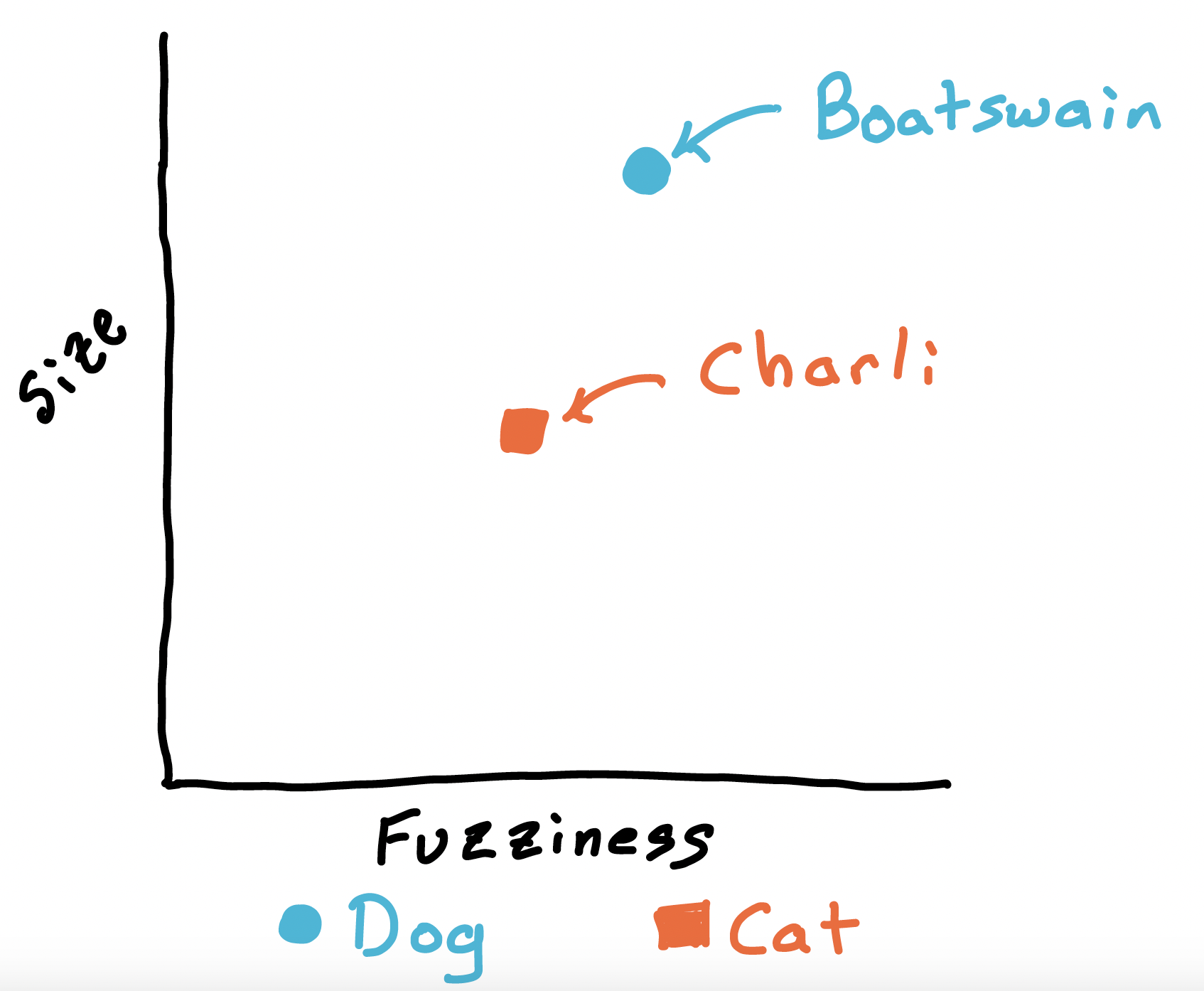
I’ve put two example animals on the chart: Boatswain the dog, and Charli the cat. We’ll represent dogs as blue circles and cats as orange squares. As Boatswain is much larger than Charli, and a tiny bit more fuzzy, he appears above and slightly to the right of Charli on the graph.

Boatswain was a dog we had when I was young, and I unfortunately don’t have a picture to share. But here’s a picture of Charli helping me prepare to teach.

Anyway, let’s add all the other dogs and cats from our training set. Then, a very basic machine learning algorithm might use the existing data to sketch a border line: on one side, it guesses “dogs”, and on the other, “cats”.

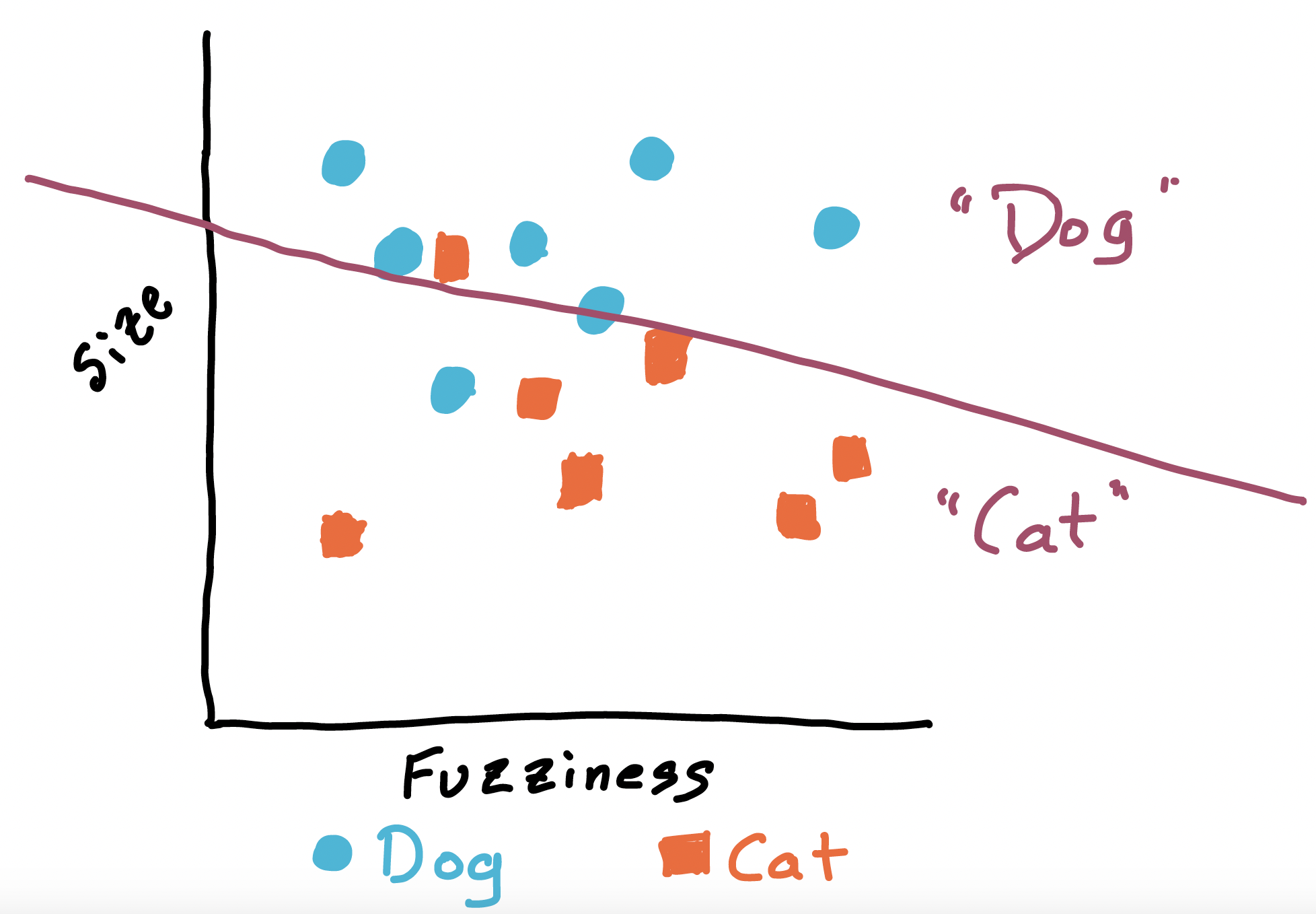
Some approaches build a more complicated border, which might be able to do better than the straight line I’ve drawn here. But this is a decent high-level sketch of how we might try to build a classifier.

Note that error is always a possibility: here we’ve misclassified one dog as a cat, and one cat as a dog. There are also a couple animals who are quite close to the line, and so might easily see their classification change if the training data are updated.

Something I wonder

This is just a toy example, but already you might see some industrial applications and potential problems that could arise from errors if the system misclassified an animal. What do you see?

Classifying Song Genre

Let’s move on to something a bit more complex, a lot more concrete, and also more related to your first project. We’re going to try to figure out what genre of music (pop, hip hop, rock, blues, country, metal, …) a song belongs to, just based on its lyrics. Here’s a few example lines from a chorus:

And here I go again, I'm drinkin' one, I'm drinkin' two
I got my heartache medication, a strong dedication
To gettin' over you, turnin' me loose
On that hardwood jukebox lost in neon time...

Do you have any guesses about what genre this song is from? If so, why?

If we believe there’s a correlation between the words in a song and its genre, it might make sense to use word counts to train a classifier. And that’s what you’ll be doing in Project 1.

Term Frequency

How might this work? Let’s consider a shorter song, which might be sung at our mascot’s birthday:

Happy Birthday to You
Happy Birthday to You
Happy Birthday Dear Bruno
Happy Birthday to You.

If we ran our word-counting program on this song, we’d get (after removing punctuation!):

{'Happy': 4,
'Birthday': 4,
'to': 3,
'Dear': 1,
'Bruno': 1,
'You': 3
}

We could get similar word count information for every song in our training set, with values for every word that appears in any song. We’ll call this the term frequency table for a given song.

From there, we can go on to imagine (although I won’t attempt to draw it!) a graph on hundreds or thousands of dimensions, where each dimension corresponds to a word. Then, a song could be put in that graph according to how many times each word appeared in it. If we believe that similar songs (by lyrics) tend to belong to similar genres, that’s a way we could build a classifier.

So far, so good, but:

• Aren’t some words more important than others?
• How would we measure distance in this mind-boggling graph?
• How do we actually go about drawing that line between genre?

We’ll answer the latter 2 questions in the project handout. For now, let’s focus on that first question; it’s vital.

Inverse Document Frequency

The country song we looked at a few minutes ago contains quite a few instances of the word “I”. For our classification purposes, do we really care as much about “I” as we do about “drinkin’” or “heartache”?

Probably not, which is where the next idea comes in. We’d like to value difference in some word counts more than others, and to do this we’ll use an idea called inverse document frequency, which essentially means finding out how common a word is in the entire training set. Words like “a” and “I” will be common; words like “drinkin’” will be less so.

TF-IDF

Putting these two ideas (Term Frequency and Inverse Document Frequency) together gives us a metric called TF-IDF. More details about this in the project handout; for now, just think about it as a sort of multiplier we’ll apply to the term frequency value that makes very common words less important. Here’s what Happy Birthday’s frequency table looks like with an IDF factor applied:

{'Happy': 4,
'Birthday': 8,
'to': 0,
'Dear': 2,
'Bruno': 8,
'You': 1.5
}

Hardly any songs use “Birthday” or “Bruno”, but many use “You” and an overwhelming number use “to”.

Discussion: Let’s think about classifiers

We saw one possible issue above: errors in classification can cause real consequences. But, it might be that an error about song genre is less dangerous than an error about animal species. There’s still the possibility of errors, though. Since machine learning can be so dependent on training data, let’s think a bit about ways that a machine-learning algorithm might be led astray, or might lead us astray.

This is a really broad question, but it needs to be!

Whenever you’re learning a new technology, it’s useful to think a bit about potential threats, biases, and other factors that might influence how you use it. You’ll be doing some reading on this concurrently with the project, but I’m glad we got to start the discussion here in class.

I want to tell you a story that might make one of the points above more real to you. During World War 2, the U.S. military was very interested in ways they could reduce the chance of aircraft loss. You can’t afford to armor an airplane as much as you might like to: the more it weighs, the harder it is to get off the ground, the less agile it is, and the more fuel it needs. The U.S. Army and Navy thought that they might be able to look at their planes after a battle and add armor to the places where they saw bullet holes.

Abraham Wald was a mathematician who was brought in to work on the project. Wald was originally from Austria, but was unable to get a University position because of anti-Semitic discrimination at the time. When Germany annexed Austria, he fled and came to the United States.

Wald noticed a problem with the military’s reasoning: something called survivorship bias, which is a kind of sampling bias. Any airplane they could examine for damage after a battle had, by definition, avoided the situation that they wanted to prevent. The others had already crashed, or exploded, or met some other fate that would prevent a careful examination.

Wald found that, rather than armoring the places where surviving planes showed damage, other places (like the fuel supply) needed to be given much more consideration. It’s estimated that Wald’s statistical work saved hundreds of lives.

Project 1

We talked a bit about Project 1; see the project handout for a more detailed presentation. The summary is that we’re asking you to build a classifier for song genre based on a corpus of training data we’ll provide.

For the classifier, you’ll use TF-IDF, and just return the genre of the nearest neighbor in the training data. There are many ways that you might define “nearest”; we’ve given you code for a metric called cosine similarity and suggest you use that. Our focus here isn’t on a deep examination of different similarity metrics, but on the engineering that frames using any metric.

Optional Supplement: Thinking More About Memory

I wanted to reinforce some of our conversations about memory. Let’s revisit what happens in memory when you create container objects like lists, sets, and dictionaries.

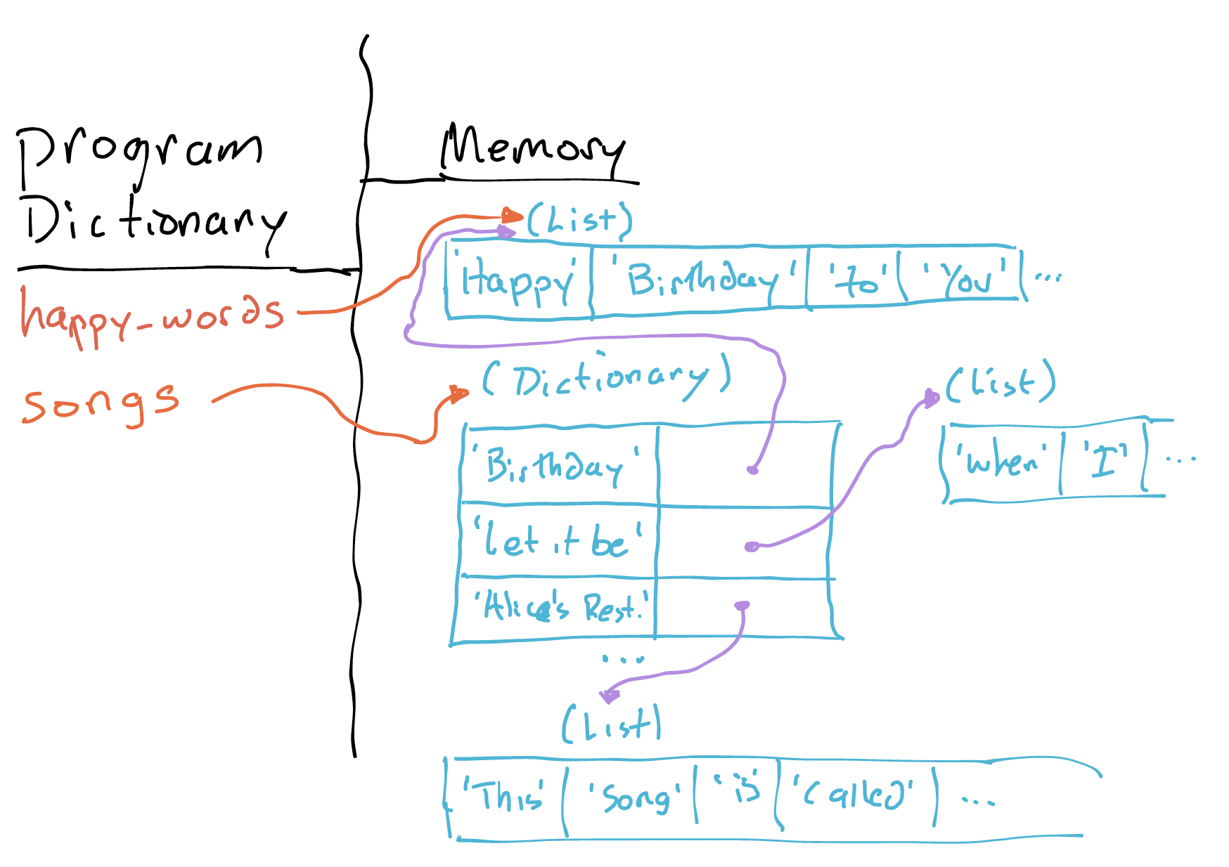
Here’s an example snapshot of part of the state of a Python program. We’ve loaded a bunch of song lyrics into memory, and in this case we’ve chosen to store them all in a dictionary (songs) indexed by the name of each song.

This snapshot was taken right after executing the line:

happy_words = songs['Birthday']

Notice what’s happened. The program knows the name happy_words now, and the name happy_words refers to a list in memory that’s storing the lyrics to “Happy Birthday”. In fact, it’s the same list that the dictionary was (and still is) storing as the value for the 'Birthday' key.

Sometimes, this is exactly the situation we want. But sometimes it isn’t. What could go wrong here? (Note that this issue, in another form, came up for some of you on the homework.)

happy_words = list(songs['Birthday'])

print(id(songs['Birthday']))
print(id(happy_words))