Program Performance (Part 2)

Today we’ll continue the discussion of runtime, and then switch to a more concrete case: figuring out how dictionaries and sets are so fast in Python. The end of these notes contains an optional exercise that is meant to reinforce the runtime material; I strongly recommend trying it out!

Note: So far we’ve seen constant, linear, and quadratic worst-case runtime. But there are others. If you see reference on a drill or on Ed to “logarithmic”, we’ll talk about how that happens in a couple weeks. But after today you should have some intuition about what it means.

Note: Keep on working on Song Analysis! Remember that the design check is due on the 24th. Just turn in the readme on gradescope and ignore any error messages it gives you.

Big-O (or asymptotic) Notation

Last time, we talked about analyzing the performance of programs. When deciding whether a function would run in constant, linear, or quadratic time, we ignored the constants and just looked at the fastest-growing (i.e., worst-scaling) term. We can define this more formally using asymptotic notation. This is also often called big-O notation (because a capital “O” is involved in the usual way of writing it).

Let’s look again at the last function we considered last time:

def distinct(l: list) -> list:
    seen = []
    for x in l:            
        if x not in seen:  # 0 + 1 + 2 + ... + (len(seen)-1) 
            seen.append(x) # once for every new element
    return seen

We decided that this function’s worst case running time is quadratic in its input (in the worst case). For a list of length $n$, we can calculate the worst-case number of operations as $\frac{n(n−1)}{2}+n+3$:

• $((n*(n−1))/2)$: when every element in l is unique, the inner membership check has to loop through the entire seen list, which grows by 1 element every iteration of the outer loop (and algebra gets us from $0 + 1 + … + (n-1)$ to this form);
• $n$: we know the append has to run once for every element of the input list in the worst case (we glossed over this last time); and
• $3$ (or some other constant): constant setup time for creating the seen list and returning from the function (Whether or not we count certain operations as the same or different, it’s still a constant).

A computer scientist would say that this function runs in $O(n^2)$ time. Said out loud, this might be pronounced: “Big Oh of n squared”.

Recall that we’re trying to collapse out factors like how fast my computer is, and focus on scaling: is there a way to formalize the idea that one algorithm is faster than another?

Why does this matter?

Question: Why do we get to treat append as something that runs in constant time? Does it necessarily do so? Might there be different ways that append works, which have different worst-case runtimes?

You’ve noticed already that the data structures you use can influence the runtime of your program. In fact, soon we’ll talk about the difference between Pyret lists and Python lists. If append were implemented with a Pyret list, it would be worst-case linear, rather than constant. This is why we saw what we did last time, between distinct via a list and distinct via a set.

Next time we’ll talk about how sets and dictionaries make this kind of fast lookup possible, and whether there are any limitations. (There are limitations.) For now, think of big-O notation as a way to quickly capture how different tools (like data structures or algorithms) scale for different purposes. If you have the option to use something in $O(n)$ instead of something in $O(n^2)$, and there are no other factors involved, you should pick the better-scaling option.

Formally Speaking

The formal definition looks like this:

If we have (mathematical, not Python!) functions $f(x)$ and $g(x)$, then $f(x)$ is in $O(g(x))$ if and only if there are constants $x_0$ and $C$ such that for all $x > x_0$, $f(x) < C g(x)$.

That is, $f(x)$ is in $O(g(x))$ if we can pick a constant $C$ so that after some point ($x_0$), $f(x)$ is always less than $C g(x)$. There may be many such $x_0$ and $C$ values that work. But if even one such pair exists, $f$ is in $O(g)$.

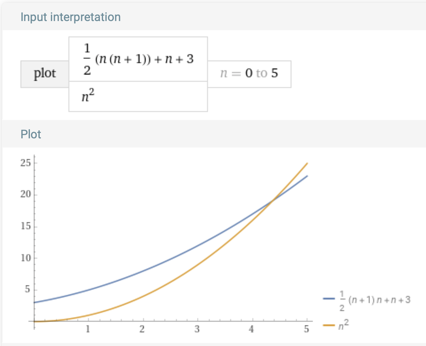
If we want to show that $\frac{n(n+1)}{2} + n + 3$ is in $O(n^2)$, our constants could be, say, $x_0 = 5$ and $C = 1$. After the list is at least $5$ elements long, $\frac{n(n+1)}{2} + n + 3$ will always be less than $1*n^2$. We could prove that using algebra, but here’s a picture motivating the argument:

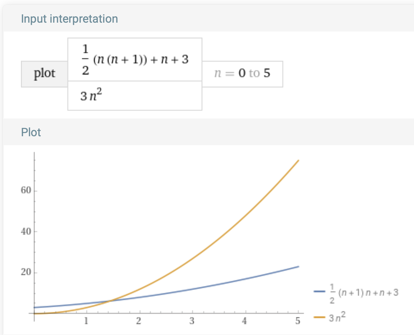
We could have picked some other values. For example, $x_0 = 2$ and $C = 3$:

Important Note: We’re using Wolfram Alpha for generating plots. Wolfram Alpha is an excellent tool which is free for personal use. Its terms allow academic use in settings such as this provided that we credit them and ideally link to the original query, which you can explore here. Note that they don’t allow, for instance, web scraping vs. their tool, so please use it responsibly!

In this class, we won’t expect you to rigorously prove that a function’s running time is in a particular big-O class. We will, though, use the notation. E.g., we’ll use $O(n)$ as a shorthand for “linear” and $O(n^2)$ as shorthand for “quadratic”. And we’ll try to be precise about whether we’re talking about “worst case”, “best case”, “average case”, etc. Don’t conflate the two ideas! “Upper bound” does not mean “worst case”. We can also put an upper bound on the best-case behavior of a program!

Also, notice that, by this definition, if a function is in $O(n)$ it is also in $O(n^2)$ and so on. The notation puts an upper limit on a function, that’s all. However, by convention, we tend to just say $O(n^2)$ by itself to mean “quadratic” rather than also saying “and not $O(n)$”.

The quick trick of looking for the largest term ($n$, $n^2$ etc.) will usually work on everything we give this semester, and in fact is a good place to start regardless. If you decide to take an algorithms course, things become both more complicated and, potentially, more interesting.

Conceptual: Let’s “Invent” Fast Dictionaries!

Last time we saw that switching from a list to a set in our distinct function produced a massive performance improvement. Today we’ll learn about why. Or, rather, we’ll invent the trick that Python sets (and dictionaries) use for ourselves! We’ll finish inventing and actually implement all this next time.

Two Inefficient Set Structures

Inefficient Structure 1

If we really wanted to, we could use Python lists to store sets. Adding an element would just mean appending a new value to the list, and checking for membership would involve a linear search through the list.

Python lists are built so that accessing any particular index takes constant time. For example, suppose we have a list called staff that stores the first names of the staff of a course:

How long does it take for Python to return 'Ben' for staff[2]? It depends on how lists are implemented! In Python, lists are contiguous blocks in memory. Python doesn’t have to count down the list elements one by one, it can just do some arithmetic and skip ahead.

This is different from how Pyret lists work. We’ll contrast the two in more detail later. For now, imagine Python lists as being written on a sheet of lined paper in memory. Element 0 is a certain distance from element 1, which is that same distance from element 2 and so on. As a result, combined with some clever hardware-design tricks, Python can get the value of staff[2] in constant time. Python doesn’t have to count down the list elements one by one, it can just do some arithmetic and skip ahead.

The trouble is that this kind of fast lookup by index doesn’t help us check for membership in the set. There’s no connection between 2 and 'Ben' except the arbitrary order in which elements were added. So let’s simplify the problem.

Inefficient Structure 2

What if, instead, the element we were searching for was the index? Suppose that we wanted to check whether a certain ID number was in our set. Then we could take advantage of how lists work in Python, and draw a picture like this, where the list elements are just True and False:

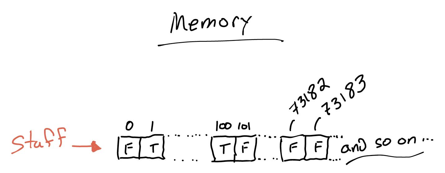
We store a True if that ID number is in the set, and False otherwise. Since Python can look up an index of a list in constant time, we can use this data structure to report on set membership in constant time—if the elements are numbers.

Aside: If we stored more than just booleans in that list, we could easily map the numeric keys to arbitrary values, much like a dictionary does. Access would remain constant time. There are also ways to address keys that aren’t just numbers, but let’s keep the discussion simple for today.

This all sounds great: it really does get us worst-case constant-time lookup!

But there’s a cost. Unless the range of possible values is small, this technique needs a colossally big list—probably more than we could fit in memory! Worse, most of it is going to be used on False values, to say “nope, nothing here!”. We’re making an extreme trade-off of space for time: allocating a list cell for every potential search key, in exchange for constant-time lookup rewards. So we need another approach.

It turns out that, from a certain point of view, the solution lies in combining these two imperfect approaches. We’ll make that connection next time.

(Optional) Programming Exercise: Rainfall

Let’s say we are tracking daily rainfall around Brown University. We want to compute the average rainfall over the period for which we have useful sensor readings. Our rainfall sensor is a bit unreliable, and reports data in a strange format. Both of these factors are things you sometimes encounter when dealing with real-world data!

In particular, our sensor data is arrives as a list of numbers like:

sensor_data = [1, 6, -2, 4, -999, 4, 5]

The -999 represents the end of the period we’re interested in. This might seem strange: why not just end the list after the first 4 value? But, for good reasons, real-world raw data formats sometimes use a “terminator” symbol like this one. It’s also possible for the -999 not to be present, in which case the entire list is our dataset.

The other negative numbers represent sensor error; we can’t really have a negative amount of rainfall. These should be scrubbed out of the dataset before we take the average.

In summary, we want to take the average of the non-negative numbers in the input list up to the first -999, if one appears. How would we solve this problem? What are the subproblems?

This time, you will drive the entire process of building the function:

• note what your input and output look like, and write a few examples to sketch the shape of the data you have and the data you need to produce;
• brainstorm the steps you might use to solve the problem (without worrying about how to actually perform them—we just did some of that above); then
• create a function skeleton, and gradually fill it in.

Since these notes are being written before lecture, it’s tough to anticipate the solutions you’ll come up with, but here are two potential solutions:

def average_rainfall(sensor_input: lst) -> float:
  number_of_readings = 0
  total_rainfall = 0
  for reading in sensor_input:
    if reading == -999:
      return total_rainfall / number_of_readings
    elif reading >= 0:
      number_of_readings += 1
      total_rainfall += reading
  return total_rainfall / number_of_readings

def list_before(l: list, item) -> list:
  result = []
  for element in l:
    if element == item:
      return result
    result.append(element)
  return result

def average_rainfall(sensor_input: lst) -> float:
  readings_in_period = list_before(sensor_input, -999)
  good_readings = [reading for reading in readings_in_period if reading >= 0]
  return sum(good_readings) / len(good_readings)

These two solutions have very different feels. One accumulates a value and count while passing through the function once, with different behaviors for different values in the list. The other produces intermediate lists that are steps on the way to the solution, before finally just computing the average value.

The first version is, in my experience, much easier to make mistakes with—and harder to build up incrementally, testing while you go. But it only traverses the list once! That means it’s faster—right?

Well, maybe.

Runtime vs. Scaling

What are the worst-case running times of each solution?

To see why this is the case, let’s look at a smaller example. This program has worst-case performance linear in the length of l:

sum = 0
for i in l:
    sum = sum + i
for i in l:
    sum = sum + i

It loops through the list twice.

But this program has quadratic performance in the length of l:

sum = 0
for i in l:
    for j in l:
        sum = sum + 1

For every element in the list, it loops again through the list.

So if you’re “counting loops” to estimate how efficient a program is, pay attention to the structure of nesting, not just the number of times you see a loop.